In this article, you will learn how to build, train, and compare an LSTM and a transformer for next-day univariate time series forecasting on real public transit data.
Topics we will cover include:
- Structuring and windowing a time series for supervised learning.
- Implementing compact LSTM and transformer architectures in PyTorch.
- Evaluating and comparing models with MAE and RMSE on held-out data.
All right, full steam ahead.
Transformer vs LSTM for Time Series: Which Works Better?
Image by Editor
Introduction
From daily weather measurements or traffic sensor readings to stock prices, time series data are present nearly everywhere. When these time series datasets become more challenging, models with a higher level of sophistication — such as ensemble methods or even deep learning architectures — can be a more convenient option than classical time series analysis and forecasting techniques.
The objective of this article is to showcase how two deep learning architectures are trained and used to handle time series data — long short term memory (LSTM) and the transformer. The main focus is not merely leveraging the models, but understanding their differences when handling time series and whether one architecture clearly outperforms the other. Basic knowledge of Python and machine learning essentials is recommended.
Problem Setup and Preparation
For this illustrative comparison, we will consider a forecasting task on a univariate time series: given the temporally ordered previous N time steps, predict the (N+1)th value.
In particular, we will use a publicly available version of the Chicago rides dataset, which contains daily recordings for bus and rail passengers in the Chicago public transit network dating back to 2001.
This initial piece of code imports the libraries and modules needed and loads the dataset. We will import pandas, NumPy, Matplotlib, and PyTorch — all for the heavy lifting — along with the scikit-learn metrics that we will rely on for evaluation.
|
import pandas as pd import numpy as np import matplotlib.pyplot as plt
import torch import torch.nn as nn from sklearn.metrics import mean_squared_error, mean_absolute_error
url = “https://data.cityofchicago.org/api/views/6iiy-9s97/rows.csv?accessType=DOWNLOAD” df = pd.read_csv(url, parse_dates=[“service_date”]) print(df.head()) |
Since the dataset contains post-COVID real data about passenger numbers — which may severely mislead the predictive power of our models due to being very differently distributed than pre-COVID data — we will filter out records from January 1, 2020 onwards.
|
df_filtered = df[df[‘service_date’] <= ‘2019-12-31’]
print(“Filtered DataFrame head:”) display(df_filtered.head())
print(“\nShape of the filtered DataFrame:”, df_filtered.shape) df = df_filtered |
A simple plot will do the job to show what the filtered data looks like:
|
df.sort_values(“service_date”, inplace=True) ts = df.set_index(“service_date”)[“total_rides”].fillna(0)
plt.plot(ts) plt.title(“CTA Daily Total Rides”) plt.show() |
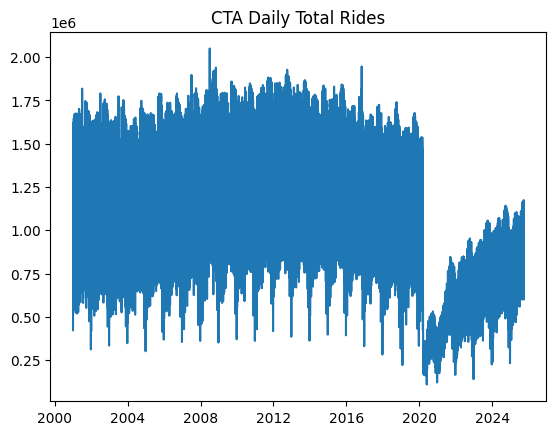
Chicago rides time series dataset plotted
Next, we split the time series data into training and test sets. Importantly, in time series forecasting tasks — unlike classification and regression — this partition cannot be done at random, but in a purely sequential fashion. In other words, all training instances come chronologically first, followed by test instances. This code takes the first 80% of the time series as a training set, and the remaining 20% for testing.
|
n = len(ts) train = ts[:int(0.8*n)] test = ts[int(0.8*n):]
train_vals = train.values.astype(float) test_vals = test.values.astype(float) |
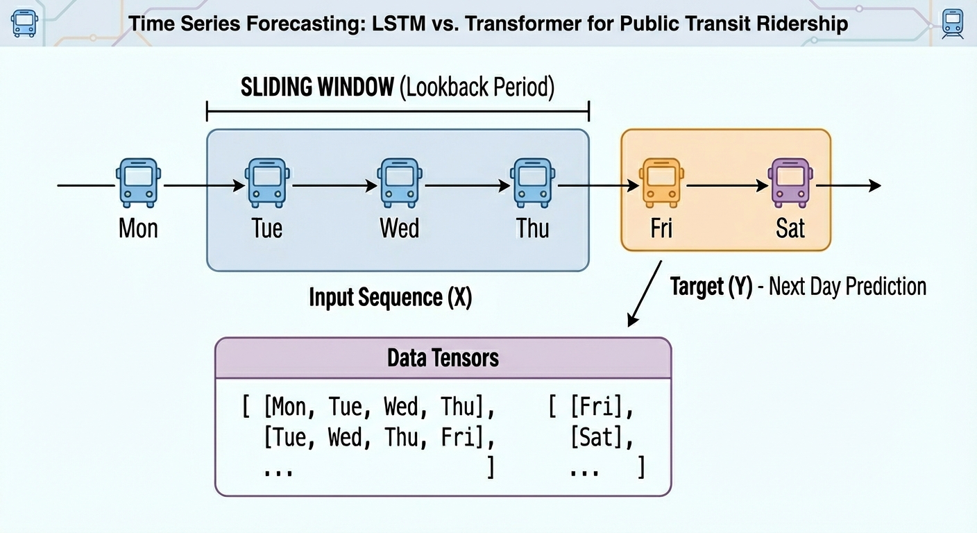
Furthermore, raw time series must be converted into labeled sequences (x, y) spanning a fixed time window to properly train neural network-based models upon them. For example, if we use a time window of N=30 days, the first instance will span the first 30 days of the time series, and the associated label to predict will be the 31st day, and so on. This gives the dataset an appropriate labeled format for supervised learning tasks without losing its important temporal meaning:
|
def create_sequences(data, seq_len=30): X, y = [], [] for i in range(len(data)–seq_len): X.append(data[i:i+seq_len]) y.append(data[i+seq_len]) return np.array(X), np.array(y)
SEQ_LEN = 30 X_train, y_train = create_sequences(train_vals, SEQ_LEN) X_test, y_test = create_sequences(test_vals, SEQ_LEN)
# Convert our formatted data into PyTorch tensors X_train = torch.tensor(X_train).float().unsqueeze(–1) y_train = torch.tensor(y_train).float().unsqueeze(–1) X_test = torch.tensor(X_test).float().unsqueeze(–1) y_test = torch.tensor(y_test).float().unsqueeze(–1) |
We are now ready to train, evaluate, and compare our LSTM and transformer models!
Model Training
We will use the PyTorch library for the modeling stage, as it provides the necessary classes to define both recurrent LSTM layers and encoder-only transformer layers suitable for predictive tasks.
First up, we have an LSTM-based RNN architecture like this:
|
class LSTMModel(nn.Module): def __init__(self, hidden=32): super().__init__() self.lstm = nn.LSTM(1, hidden, batch_first=True) self.fc = nn.Linear(hidden, 1)
def forward(self, x): out, _ = self.lstm(x) return self.fc(out[:, –1])
lstm_model = LSTMModel() |
As for the encoder-only transformer for next-day time series forecasting, we have:
|
class SimpleTransformer(nn.Module): def __init__(self, d_model=32, nhead=4): super().__init__() self.embed = nn.Linear(1, d_model) enc_layer = nn.TransformerEncoderLayer(d_model=d_model, nhead=nhead, batch_first=True) self.transformer = nn.TransformerEncoder(enc_layer, num_layers=1) self.fc = nn.Linear(d_model, 1)
def forward(self, x): x = self.embed(x) x = self.transformer(x) return self.fc(x[:, –1])
transformer_model = SimpleTransformer() |
Note that the last layer in both architectures follows a similar pattern: its input shape is the hidden representation dimensionality (32 in our example), and one single neuron is used to perform a single forecast of the next-day total rides.
Time to train the models and evaluate both models’ performance with the test data:
|
def train(model, X, y, epochs=10): model.train() opt = torch.optim.Adam(model.parameters(), lr=1e–3) loss_fn = nn.MSELoss()
for epoch in range(epochs): opt.zero_grad() out = model(X) loss = loss_fn(out, y) loss.backward() opt.step() return model
lstm_model = train(lstm_model, X_train, y_train) transformer_model = train(transformer_model, X_train, y_train) |
We will compare how the models performed for a univariate time series forecasting task using two common metrics: mean absolute error (MAE) and root mean squared error (RMSE).
|
lstm_model.eval() transformer_model.eval()
pred_lstm = lstm_model(X_test).detach().numpy().flatten() pred_trans = transformer_model(X_test).detach().numpy().flatten() true_vals = y_test.numpy().flatten()
rmse_lstm = np.sqrt(mean_squared_error(true_vals, pred_lstm)) mae_lstm = mean_absolute_error(true_vals, pred_lstm)
rmse_trans = np.sqrt(mean_squared_error(true_vals, pred_trans)) mae_trans = mean_absolute_error(true_vals, pred_trans)
print(f“LSTM RMSE={rmse_lstm:.1f}, MAE={mae_lstm:.1f}”) print(f“Trans RMSE={rmse_trans:.1f}, MAE={mae_trans:.1f}”) |
Results Discussion
Here are the results we obtained:
|
LSTM RMSE=1350000.8, MAE=1297517.9 Trans RMSE=1349997.3, MAE=1297514.1 |
The results are incredibly similar between the two models, making it difficult to determine whether one is better than the other (if we look closely, the transformer performs a tiny bit better, but the difference is truly negligible).
Why are the results so similar? Univariate time series forecasting on data that follow a reasonably consistent pattern over time, such as the dataset we consider, can yield similar results across these models because both have enough capacity to solve this problem — even though the complexity of each architecture here is intentionally minimal. I suggest you try the entire process again without filtering the post-COVID instances, keeping the same 80/20 ratio for training and testing over the entire original dataset, and see if the difference between the two models increases (feel free to comment below with your findings).
Besides, the forecasting task is very short-term: we are just predicting the next-day value, instead of having a more complex label set y that spans a subsequent time window to the one considered for inputs X. If we predicted values 30 days ahead, the difference between the models’ errors would likely widen, with the transformer arguably outperforming the LSTM (although this might not always be the case).
Wrapping Up
This article showcased how to address a time series forecasting task with two different deep learning architectures: LSTM and the transformer. We guided you through the entire process, from obtaining the data to training the models, evaluating them, comparing, and interpreting results.